FINANCIAL FUNCTION IN EXCEL

1 – FUTURE VALUE (FV) : FINANCIAL FUNCTION IN EXCEL 

If you want to find out the future value of a particular investment which has a constant interest rate and periodic payment, use the following formula –

FV (Rate, Nper, [Pmt], PV, [Type])

• Rate = It is the interest rate/period
• Nper = Number of periods
• [Pmt] = Payment/period
• PV = Present Value
• [Type] = When the payment is made (if nothing is mentioned, it’s assumed that the payment has been made at the end of the period)

FV EXAMPLE

A has invested US $100 in 2016. The payment has been made yearly. The interest rate is 10% p.a. What would be the FV in 2019?

Solution: In excel, we will put the equation as follows –

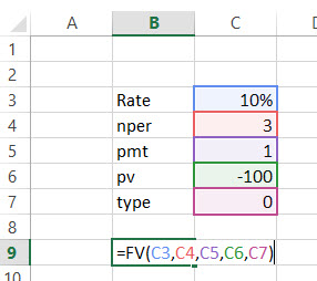
= FV (10%, 3, 1, – 100)

= US $129.79

2 – FVSCHEDULE  : FINANCIAL FUNCTION IN EXCEL 

This financial function is important when you need to calculate the future value with the variable interest rate. Have a look at the function below –

FVSCHEDULE = (Principal, Schedule)

• Principal = Principal is the present value of a particular investment
• Schedule = A series of interest rate put together (in case of excel, we will use different boxes and select the range)

FVSCHEDULE EXAMPLE:

M has invested US $100 at the end of 2016. It is expected that the interest rate will change every year. In 2017, 2018 & 2019, the interest rates would be 4%, 6% & 5% respectively. What would be the FV in 2019?

Solution: In excel, we will do the following –

= FVSCHEDULE (C1, C2:C4)

= US $115.752

3 – PRESENT VALUE (PV) : FINANCIAL FUNCTION IN EXCEL 

If you know how to calculate FV, it’s easier for you to find out PV. Here’s how –

PV = (Rate, Nper, [Pmt], FV, [Type])

• Rate = It is the interest rate/period
• Nper = Number of periods
• [Pmt] = Payment/period
• FV = Future Value
• [Type] = When the payment is made (if nothing is mentioned, it’s assumed that the payment has been made at the end of the period)

PV EXAMPLE:

The future value of an investment is US $100 in 2019. The payment has been made yearly. The interest rate is 10% p.a. What would be the PV as of now?

Solution: In excel, we will put the equation as follows –

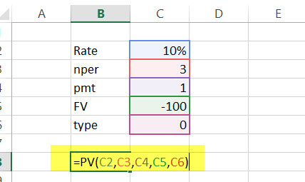
= PV (10%, 3, 1, – 100)

= US $72.64

4 – NET PRESENT VALUE (NPV) : FINANCIAL FUNCTION IN EXCEL 

Net Present Value is the sum total of positive and negative cash flows over the years. Here’s how we will represent it in excel –

NPV = (Rate, Value 1, [Value 2], [Value 3]…)

• Rate = Discount rate for a period
• Value 1, [Value 2], [Value 3]… = Positive or negative cash flows
• Here, negative values would be considered as payments and positive values would be treated as inflows.

NPV EXAMPLE

Here is a series of data from which we need to find NPV –

Details	In US $
Rate of Discount	5%
Initial Investment	-1000
Return from 1st year	300
Return from 2nd year	400
Return from 3rd year	400
Return from 4th year	300

Find out the NPV.

Solution: In Excel, we will do the following –

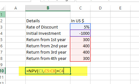
=NPV (5%, B4:B7) + B3

= US $240.87

5 – XNPV  : FINANCIAL FUNCTION IN EXCEL 

This financial function is similar as the NPV with a twist. Here the payment and income are not periodic. Rather specific dates are mentioned for each payment and income. Here’s how we will calculate it –

XNPV = (Rate, Values, Dates)

• Rate = Discount rate for a period
• Values = Positive or negative cash flows (an array of values)
• Dates = Specific dates (an array of dates)

XNPV EXAMPLE

Here is a series of data from which we need to find NPV –

Details	In US $	Dates
Rate of Discount	5%
Initial Investment	-1000	1st December, 2011
Return from 1st year	300	1st January, 2012
Return from 2nd year	400	1st February, 2013
Return from 3rd year	400	1st March, 2014
Return from 4th year	300	1st April, 2015

Solution: In excel, we will do as following –

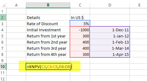
=XNPV (5%, B2:B6, C2:C6)

= US$289.90

6 – PMT : FINANCIAL FUNCTION IN EXCEL 

In excel, PMT denotes the periodical payment required to pay off for a particular period of time with a constant interest rate. Let’s have a look at how to calculate it in excel –

PMT = (Rate, Nper, PV, [FV], [Type])

• Rate = It is the interest rate/period
• Nper = Number of periods
• PV = Present Value
• [FV] = An optional argument which is about the future value of a loan (if nothing is mentioned, FV is considered as “0”)
• [Type] = When the payment is made (if nothing is mentioned, it’s assumed that the payment has been made at the end of the period)

PMT EXAMPLE

US $1000 need to be paid in full in 3 years. Interest rate is 10% p.a. and the payment needs to be done yearly. Find out the PMT.

Solution: In excel, we will compute it in the following manner –

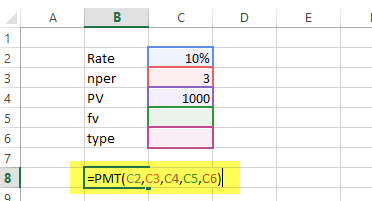
= PMT (10%, 3, 1000)

= – 402.11

2nd year,

=PPMT (10%, 2, 3, 1000)

= US $-332.33

financial function